 Non-profit
Joint-stock
Company


Department of Physics
PHYSICS OF ELECTROMAGNETIC WAVES
Lecture notes for students of specialty
5В071900 - Radio engineering, electronics and telecommunications
Almaty 2017
AUTHORS: M. Sh. Karsybayev, G.S. Asanov. Physics of electromagnetic waves. Lecture notes for students of specialty 5В071900 - Radio engineering, electronics and telecommunications. - Almaty: AUPET, 2017. – 50 p.
A brief summary of lectures on course of «Physics of electromagnetic waves» for radio engineering, electronics and telecommunications specialties of a bachelor degree is stated.
The lectures abstract «Physics of electromagnetic waves» is necessary for methodical maintenance of educational process on course and can be used as a distributing material on lecture employment and also in self-study work above a theoretical material by preparation to practical and laboratory classes and examinations.
Fig. - 33 , tab. - 3, bibl. - 8 items.
The reviewer: assistant professor Tuzelbaev B.I.
Almaty University of power engineering and telecommunications is printed under the additional plan of the edition of non-profit joint-stock company.
© NPJSC “Almaty university of power engineering and telecommunications”, 2017
Contents
Introduction
The abstract of lectures on« Physics of electromagnetic waves» represents a statement of the contents of lectures material on this discipline and is intended for students who are educated under programs of a bachelor degree at faculty FRTC. A course of « Physics of electromagnetic waves» includes some sections of classical and modern physics. Clear physical and world outlook interpretation of classical and modern physics forms at students an ability to rearrange the thinking to perception of inevitable transformations of old scientific and technical representations in essentially new. In each lecture the basic questions of a theme in their logic connection and structural integrity but without detailed study of mathematical calculations or examples are reflected. Therefore the given educational and methodical work can and should form only rough basis for educational activity of the student by preparation for practical employment, borderline and final control.
1 Lecture №1. Maxwell's equations
Lecture content: essence of electromagnetic induction phenomenon and Maxwell’s equations as classical theory.
Lecture aim: to give students basic knowledge of:
- phenomenon and law of electromagnetic induction, displacement current;
- to reveal physical meaning of Maxwell’s equations which form the basis of the unified theory of classical electrodynamics.
1.1 The phenomenon and the law of an electromagnetic induction
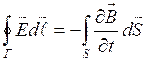
In 1831 M. Faraday had discovered the phenomenon of an electromagnetic induction: the induced current emerges in the closed conducting loop at a change of magnetic induction flux penetrating this loop.
 The induced
current can be caused in two ways: first way - moving of framework Р in
created by coil K with a current magnetic field and galvanometer G in framework
Р will indicate induced current; second way - framework Р is
motionless but the magnetic field changes. We can see these ways in figure 1.1.
There are a coil K with a source and a rheostat for current change; a loop Р closed on the galvanometer G.
The induced
current can be caused in two ways: first way - moving of framework Р in
created by coil K with a current magnetic field and galvanometer G in framework
Р will indicate induced current; second way - framework Р is
motionless but the magnetic field changes. We can see these ways in figure 1.1.
There are a coil K with a source and a rheostat for current change; a loop Р closed on the galvanometer G.
Figure 1.1
Rule (law) of Lenz: The direction of current induced in a conductor by a changing magnetic field will be such that it will create a field that opposes the change that produced it. It means that the induced current creates its magnetic flux interfering change of an initial magnetic flux causing an induced current.
Rule of Lenz corresponds to position according to which the system aspires to counteract change of its condition. Electromagnetic inertia is manifested in it. Rule of Lenz follows from the law of conservation of energy.
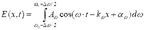
Law of an electromagnetic induction:
![]() . (1.1)
. (1.1)
Electromotive
force (EMF) ![]() of
electromagnetic induction is equal to the speed of magnetic flux change taken
with the opposite sign. Sign "minus" is physically caused by Lenz
rule.
of
electromagnetic induction is equal to the speed of magnetic flux change taken
with the opposite sign. Sign "minus" is physically caused by Lenz
rule.
Let’s consider two cases specified mentioned above:
а) Law of an electromagnetic induction at movement of a loop in a constant magnetic field.
EMF of electromagnetic induction
![]() ,
(1.2)
,
(1.2)
where ![]() is
field of external force and
is
field of external force and ![]() is
an increment of a loop P area per time equals to
is
an increment of a loop P area per time equals to ![]() ,
then
,
then ![]() and
and ![]() .
.
b) A vortex electric field.
In second case a loop P is motionless in a variable magnetic field. Question of principle appears: what is the nature of outside forces?
There
are only two forces: electric ![]() and magnetic
and magnetic ![]() . The second
force equals zero, therefore remains only first force: the induced current is
caused by a variable electric field
. The second
force equals zero, therefore remains only first force: the induced current is
caused by a variable electric field ![]() arising in a loop.
arising in a loop.
According to first Maxwell's hypothesis: magnetic field changing in time leads to occurrence in space of a vortex electric field.
![]() and
and ![]() . (1.3)
. (1.3)
Show
it: ![]() or
or  .
.
Under Stokes theorem
 and
whence
and
whence  .
.
1.2 Displacement current
Second hypothesis of Maxwell: the electric field changing in time creates a magnetic field. Maxwell has entered concept of a displacement current which in addition to conductivity current creates a magnetic field.
The density of a displacement current is
![]() . (1.4)
. (1.4)
Density of a full current
![]() . (1.5)
. (1.5)
Thus
![]() (1.6)
(1.6)
and
![]() . (1.7)
. (1.7)
For general case (non-stationary fields) a time change of an electric field generates a variable magnetic field.
1.3 System of Maxwell's equations (in motionless environments)
It represents, in essence, the uniform theory of the electric and magnetic phenomena. In the integrated form:
 ; (1.8)
 ;
(1.9)
;
(1.9)
 ;
(1.10)
;
(1.10)
![]() . (1.11)
. (1.11)
Let's
express physical sense of each equation. From expressions for ![]() and
and ![]() circulation
follows that electric and magnetic fields cannot be considered as independent:
change in time of one of the fields lead to occurrence of another. Only the set
of these fields representing a uniform electromagnetic field therefore
is meaningful.
circulation
follows that electric and magnetic fields cannot be considered as independent:
change in time of one of the fields lead to occurrence of another. Only the set
of these fields representing a uniform electromagnetic field therefore
is meaningful.
If
fields are permanent, i.e. ![]() and
and ![]() equations of
Maxwell can be rewritten as:
equations of
Maxwell can be rewritten as:
![]() ,
, ![]() ,
, ![]() ,
, ![]() . (1.12)
. (1.12)
In this case fields are independent and can be studied separately.
In the differential form the equations (1.8) - (1.11) will be the following :
![]() ;
(1.13)
;
(1.13)
![]() ;
(1.14)
;
(1.14)
![]() ;
(1.15)
;
(1.15)
![]() .
(1.16)
.
(1.16)
Let's
specify the physical meaning of these equations. Besides these equations not
only express fundamental laws of an electromagnetic field but also allow to
find fields ![]() at
their integration and
at
their integration and ![]() .
.
In the integrated form of Maxwell’s equations are more common since they are fair on border of environments. The differential form has limitation - all sizes in space and time change only continuously. Therefore they are supplemented with boundary conditions:
![]() ; (1.17)
; (1.17)
![]() (1.18)
(1.18)
and the medium equations:
![]() ,
, ![]() ,
, ![]() . (1.19)
. (1.19)
Specify the general properties of equations:
1)
Maxwell's equations are linear, i.e. they contain only the first derivatives of
![]() and
and ![]() on coordinates
and time and the first degrees of ρ and
on coordinates
and time and the first degrees of ρ and ![]() ;
;
2) they contain the equation of continuity i.e. the law of conservation electric charge;
3) they are carried out in all inertial frames of reference, i.e. are relativistic invariant;
4) they are not symmetric concerning electric and magnetic fields for the lack of magnetic charges in the nature. But in the neutral homogeneous non-conducting environment where ρ =0 and j=0 Maxwell's equations become symmetric (accepting a sign):
![]()
![]() . (1.20)
. (1.20)
1.4 A relativity of electric and magnetic fields
For an electromagnetic field the Einstein’s principle of relativity as the fact of propagation of electromagnetic waves in vacuum in all frames of reference with identical speed is not compatible with a Galilee’s principle of relativity.
From relativity principle follows that separate consideration of electric and magnetic fields has a relative sense. So if the electric field is created by system of motionless charges these charges being motionless concerning one inertial frame of reference moves concerning another frame and will generate hence beside an electric also a magnetic field. Similarly motionless concerning one inertial frame of reference a conductor with a direct current, raising in each point of space the constant magnetic field, goes concerning other inertial systems and the variable magnetic field created by it raises a vortex electric field.
2 Lecture №2. Oscillatory processes
Lectures content: definitions and general characteristics of various types of oscillations in oscillatory circuit.
Lecture aim: to give students basic knowledge of:
- overall concept and classification of oscillations;
- general description of harmonic oscillations;
- general equation of oscillatory circuit and modes therein.
2.1 Oscillations
Oscillations are observed in systems of various natures. Oscillations refer to processes which precisely or approximately repeat through identical time intervals. Irrespective of the nature oscillations obey the same laws, therefore for their description identical mathematical device is used.
Free, forced oscillations and self-oscillations, etc. are distinguished.
Free (or natural) oscillations are oscillations which:
а) result from initial displacement from balanced state;
b) occur freely.
According to form harmonic and saw tooth oscillations, П-shaped and others are distinguished.
Periodic oscillations of value ξ(t) refer to harmonic if they occur under the law of sine or cosine:
ξ (t) =A cos (ωt + φ0),
where ξ(t) characterizes change of any physical quantity (current, voltage, etc.);
A - amplitude of oscillations, i.e. the maximal displacement of physical quantity.
Value of oscillating quantity is ξ (t) at an arbitrary moment of time t is defined by oscillation phase value:
φ (t) = ωt + φ0,
where ω - cyclic (circular) frequency;
φ0 - initial phase, that is phase at the moment of time t=0.
ω =2 πν =2 π ⁄ Т,
where ν =1⁄Т is frequency of oscillations which defines as number of oscillations per unit time and is measured in hertz (Hz). 1 Hz=1 s-1.
Period of oscillation Т is a period of time when one full -wave oscillation happens. During the time interval equal to period Т, phase of harmonic oscillations changes on 2 π.
Amplitude and initial phase are defined by initial conditions, and frequency (or period) – by parameters of oscillatory system.
Let's find the first and second derivatives of physical quantity oscillating according to harmonic law ξ (t):
d ξ/dt =-Aωsin (ωt + φ 0) =Acos (ωt + φ0 + π/2);
d2 ξ/dt2 =-Aω2cos (ωt + φ 0) =Aω2cos (ωt + φ0 + π).
In case of mechanical oscillations the value ξ makes sense of oscillating material point coordinate and dξ/dt and d2ξ/dt2 according to its speed and acceleration.
d2 ξ/dt2 + ω2 ξ (t) =0.
Differential equation of harmonic oscillations of the second order, homogeneous, linear concerning function ξ(t).
2.2 Electrical oscillations
Electrical
oscillations are observed in the real oscillatory contour
consisting of active resistance R, condenser C and the coil of inductance L.
For supervision of undamped oscillations in a contour it is necessary to
connect external periodic EMF![]() .
.
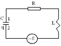 The
general equation for a contour 1RL2 can be received with the help of the Ohm’s
law:
The
general equation for a contour 1RL2 can be received with the help of the Ohm’s
law:
![]() ,
,
if the condition of quasi-stationarity is
satisfied: ![]()
sing ![]() and
and ![]() we shall receive
we shall receive
Figure 2.1 the general equation of an oscillatory contour:
![]() or
or ![]() . (2.1)
. (2.1)
Having divided
by ![]() and
with the account
and
with the account ![]() ;
;
![]() ;
; ![]() we shall receive:
we shall receive:
![]() .
(2.2)
.
(2.2)
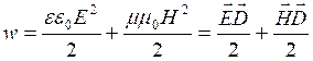
We shall consider characteristics of all kinds of oscillations in two tables.
In
table 1 the data for free oscillations without damping in an ideal oscillatory
contour with R = 0, ![]() are shown.
are shown.
Table 1
|
Differential Equation |
The solution |
Period, frequency |
|
|
|
frequency of self-contour oscillations |
In table 2 the data for
free fading oscillations in an oscillatory contour with R![]() 0,
ε=0 are
shown.
0,
ε=0 are
shown.
Table 2
|
Differential Equations |
The solution |
Characteristics |
|
|
|
|
In table 3 the data for
the forced electric oscillations in an oscillatory contour are shown for R![]() 0,
ε
0,
ε![]() 0.
0.
Table 3
|
Differential equations |
The solution |
|
electromotive force |
|
Let's write down for the forced electrical oscillations time dependence of voltage on R, C and L:
![]() ;
;
![]() ;
(2.3)
;
(2.3)
![]() .
.
These formulas allow to construct the vector diagram (figure 2) having represented amplitudes of voltage in view of their phases.
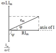
Figure 2.2
2.3 Alternating electric current
Under
influence of an external voltage ![]() the current in a circuit of an
alternating current changes under the law
the current in a circuit of an
alternating current changes under the law ![]() . Here expressions for
. Here expressions for
![]() (2.4)
(2.4)
and
![]() (2.5)
(2.5)
coincide with the solution for the forced electric oscillations.
For an alternating current the Ohm’s law is expressed as
![]() , (2.6)
, (2.6)
where
![]() is the
full resistance or an impedance of a circuit.
is the
full resistance or an impedance of a circuit.
It is
visible that at ![]() impedance
is minimal and equals to active resistance R. The quantity
impedance
is minimal and equals to active resistance R. The quantity ![]() is named by
reactive resistance,
is named by
reactive resistance, ![]() is an inductive resistance, and
is an inductive resistance, and ![]() is a
capacitance resistance. Basic difference of reactive resistance from active
that the Joule heat is not exuded on it.
is a
capacitance resistance. Basic difference of reactive resistance from active
that the Joule heat is not exuded on it.
Average for the period of oscillations value of the power exuded in a circuit of an alternating current equals
![]() .
(2.7)
.
(2.7)
The
direct current ![]() develops
same capacity. The quantities
develops
same capacity. The quantities ![]() and
and ![]() are named effective
values
of a current and a voltage. All ammeters and voltmeters in laboratories are
graduated only on effective values of a current and a voltage.
are named effective
values
of a current and a voltage. All ammeters and voltmeters in laboratories are
graduated only on effective values of a current and a voltage.
Multiplier ![]() is named factor of power
and dependence of capacity from
is named factor of power
and dependence of capacity from ![]() is
necessary for taking into account at designing a transmission line on an
alternating current.
is
necessary for taking into account at designing a transmission line on an
alternating current.
3 Lecture №3. Electromagnetic waves
Lectures сontent: existence of electromagnetic waves as consequence of Maxwell’s equations and their properties.
Lecture aim:
give students basic knowledge of:
- wave equation for electromagnetic waves;
- properties of electromagnetic waves;
- energy and a pulse of an electromagnetic field. Poynting vector;
- radiation of a dipole.
3.1 Wave equation
The
electromagnetic field can exist independently without electric charges
and currents! It follows from a presence of a displacement current ![]() in the
Maxwell's equations, i.e. a variable electric field
in the
Maxwell's equations, i.e. a variable electric field![]() generates
variable magnetic field
generates
variable magnetic field ![]() and a variable magnetic field and
vice versa. Such mutual transformation occurs continuously therefore they are
kept and distributed in space. Change of a state of a field has wave
character, i.e. fields extending in space are electromagnetic waves. It
proves to be true by the fact of reception of the wave equation from Maxwell's
equations.
and a variable magnetic field and
vice versa. Such mutual transformation occurs continuously therefore they are
kept and distributed in space. Change of a state of a field has wave
character, i.e. fields extending in space are electromagnetic waves. It
proves to be true by the fact of reception of the wave equation from Maxwell's
equations.
For
homogeneous neutral (![]() ) and non-conducting (
) and non-conducting (![]() ) medium at
constant
) medium at
constant ![]() and
and ![]() with the
account
with the
account ![]() also
also
![]() we
shall write down equations of Maxwell in a differential form:
we
shall write down equations of Maxwell in a differential form:
![]() ;
(3.1)
;
(3.1)
![]() ;
(3.2)
;
(3.2)
![]() ;
(3.3)
;
(3.3)
![]() .
(3.4)
.
(3.4)
Let's take a rotor from both parts of the equation (3.1):
 .
(3.5)
.
(3.5)
In the left part a double vector product is opened out by a rule
![]() that is
that is ![]() .
.
Taking
into account (3.3) and![]() , in the left part we
have:
, in the left part we
have:
![]() .
.
In
the right part we shall change places of sequence of differentiation on
coordinates and on time: ![]() and using (3.2) we
shall receive:
and using (3.2) we
shall receive:
 .
.
Having equated the left and right parts we shall receive the wave equation for:
 (3.6)
(3.6)
Similarly for:
 (3.7)
(3.7)
The
wave equations (3.6) and (3.7) specify an existence of the electromagnetic
waves propagating with phase speed ![]() .
.
3.2 Properties of electromagnetic waves
The basic properties of electromagnetic waves follow from Maxwell's equations:
а) in
vacuum they are always distributed with a speed ![]() .
.
In the non-conducting and not ferromagnetic environment
![]() ,
where
,
where ![]() . (3.8).
. (3.8).
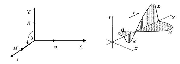
Figure 3.1 Figure 3.2
b) the
vectors ![]() are
mutually perpendicular, i.e. electromagnetic waves cross-section, and form правовинтовую system.
It - internal property of an electromagnetic wave (figure 3.1).
are
mutually perpendicular, i.e. electromagnetic waves cross-section, and form правовинтовую system.
It - internal property of an electromagnetic wave (figure 3.1).
c) the
vectors ![]() and
and ![]() always
oscillate in identical phases (figure 3.2). Between instant values
always
oscillate in identical phases (figure 3.2). Between instant values ![]() and
and ![]() in
any point next connection takes place:
in
any point next connection takes place:
![]() or
or
![]() .
(3.9)
.
(3.9)
3.3 Vector Poyting
The density of energy of an electromagnetic field is equal to the sum of density of energy for electric and magnetic fields (at absence of ferroelectrics and ferromagnets):
 . (3.10)
Taking
into account (3.9) we shall receive that ![]() for each moment of time then
for each moment of time then
![]() .
.
Poynting has entered concept of a vector of density of a flux of energy:
![]() (3.11)
(3.11)
Flux Ф of electromagnetic energy through surface F is equal
![]() .
(3.12)
.
(3.12)
3.4 Pressure and momentum of an electromagnetic field
Pressure of an electromagnetic wave upon a body on which it results from influence of a magnetic field of a wave on the electric currents raised by an electric field of the same wave.
Let the
electromagnetic wave falls on absorbing body then Joule's heat arises in it
with volumetric density σЕ2, i.e. e. ![]() and the absorbing environment
possesses conductivity. In such environment the electric field of a wave raises
an electric current with density
and the absorbing environment
possesses conductivity. In such environment the electric field of a wave raises
an electric current with density![]() . Then
on unit of volume of environment Ampere's force
. Then
on unit of volume of environment Ampere's force ![]() operates in a direction of a wave. This force
also causes pressure of an electromagnetic wave. If there is no absorption,
σ = 0 and pressure are not present. At full reflection of a wave pressure
grows twice.
operates in a direction of a wave. This force
also causes pressure of an electromagnetic wave. If there is no absorption,
σ = 0 and pressure are not present. At full reflection of a wave pressure
grows twice.
Pressure is equal:
![]() . (3.13)
. (3.13)
In (3.13)
![]() is
an average value of volumetric density of energy,
is
an average value of volumetric density of energy, ![]() is a factor of
reflection.
is a factor of
reflection.
The
density of a momentum is equal
![]() that is similar to expression
that is similar to expression ![]() for
a photon momentum.
for
a photon momentum.
3.4 Dipole radiation
An
electric dipole is the system from two equal on size but opposite on a sign
charges divided in some distance![]() .
.
If an electric dipole oscillates it radiates electromagnetic waves.
Change of its moment with time can be expressed as:
![]() . (3.14)
. (3.14)
Let's
consider an elementary dipole (figure 3.3). For it ![]() . We have
. We have ![]() in a wave
zone.
in a wave
zone.
For a
spherical wave ![]()
Hence
intensity of a wave ![]() is inversely proportional to a square
of distance from a radiator and depends on θ.
is inversely proportional to a square
of distance from a radiator and depends on θ.
The diagram of a dipole radiation in polar coordinates looks like (figure 3.4).
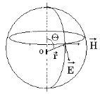
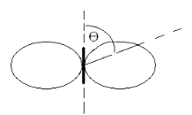
Figure 3.4 Figure 3.3
The
power of radiation![]() . We have
. We have ![]() from (3.14). Then
from (3.14). Then
![]() .
(3.15)
.
(3.15)
Let's
average on time ![]() . (3.16)
. (3.16)
From (3.14): ![]() ,
,
where a is an acceleration of oscillating charge .
Then the power of radiation is ![]() .
.
4 Lecture №4. Light as an electromagnetic wave. Light Interference
Lecture content: wave properties of light, intensity of light optical path length, interference of light waves
Lecture aim:
give students basic knowledge of:
- light nature and its wave properties;- principle the Farm and laws of geometrical optics;- coherent waves and interference of light;- methods of supervision of light interference.
4.1 Main parameters of light wave
Light wave possesses corpuscular-wave dualism: light proves а) as an electromagnetic wave and b) as a stream of particles - photons. The first case is considered (examined) in the wave optics, the second - in quantum optics.
From
two vectors ![]() and
and ![]() the basic
influence (photochemical, photo-electric, physiological, etc.) renders a
light vector
the basic
influence (photochemical, photo-electric, physiological, etc.) renders a
light vector![]() .
.
![]() .
(4.1)
.
(4.1)
Let's enter an absolute parameter of refraction of medium
![]() .
(4.2)
.
(4.2)
Taking into account
speed of electromagnetic wave ![]() ,
we shall receive
,
we shall receive
![]() .
(4.3)
.
(4.3)
This
parity connects optical properties (n) of a medium with electric (ε) and
magnetic. For transparent substances, as a rule, ![]() then
then ![]() .
.
![]() characterizes the optical density of
substance.
characterizes the optical density of
substance.
Range
of ![]() seen
light in vacuum: (3,8-7,6)10-7 m = 0,38-0,76
microns.
seen
light in vacuum: (3,8-7,6)10-7 m = 0,38-0,76
microns.
In the medium
![]() ,
i.e.
,
i.e. ![]() .
(4.4)
.
(4.4)
Frequency is
defined as ![]() and
has the order about 1015 Hz.
and
has the order about 1015 Hz.
Intensity of light is defined as average on time value of density of energy flow:
![]() .
(4.5)
.
(4.5)
Note one more useful formula I ~A2.
4.2 Optical path length
 In a
limiting case
In a
limiting case ![]() a
transition to geometrical (beam) optics takes place. In its basis are 4 laws:
a
transition to geometrical (beam) optics takes place. In its basis are 4 laws:
1) rectilinear propagation of light;
2) independence of light beams;
3) reflections;
4) refractions and a Fermat's principle: light passes on a way with minimal τ.
Let's enter optical path length:
 .
(4.6)
.
(4.6)
Figure 4.1
In
a homogeneous medium ![]() then
then![]() , i.e. light
passes on a way with minimal L.
, i.e. light
passes on a way with minimal L.
From a Fermat’s principle follows the law of convertibility of light beams: if a beam passes on the some way it will pass in an opposite direction to the same way as in direct (figure 4.1).
The
phenomenon
of total internal reflection follows from the law of refraction:
if light passes from denser optical medium (![]() ) into less dense medium and the angle of
falling reaches a limiting angle
) into less dense medium and the angle of
falling reaches a limiting angle ![]() it
will not penetrate into the second medium.
it
will not penetrate into the second medium.
4.3 Interference of light waves
Let two light waves are propagated in one direction:
![]() and
and ![]() .
.
Then![]() , where
, where![]() .
.
If ![]() waves are coherent. Let's give next definition: waves for which
waves are coherent. Let's give next definition: waves for which
![]() and the
difference of phases is constant in time refer to coherent.
and the
difference of phases is constant in time refer to coherent.
For incoherent waves δ continuously changes and its average on time value equally 0 therefore
![]() or
or ![]() , i.е.
intensities are added up.
, i.е.
intensities are added up.
For coherent waves
![]() .
(4.7)
.
(4.7)
The phenomenon of redistribution of a light flow in space therefore in one places there are maxima of intensity and in others - minima refers to as an interference.
Example:
Let ![]() . From (3.1) follows:
. From (3.1) follows: ![]() . All
natural light sources are incoherent. An explanation:
Radiation of bodies consists of the waves which are emitted by many atoms. Every atom emits a train of waves
with a duration of
the order
. All
natural light sources are incoherent. An explanation:
Radiation of bodies consists of the waves which are emitted by many atoms. Every atom emits a train of waves
with a duration of
the order ![]() s and
extent of the order
s and
extent of the order ![]() = 3 (m).
= 3 (m).
After a time of radiation of a group
of atoms τ is replaced by the
radiation of the other group of atoms. Phase of different trains
of waves even
from one atom is
not connected, i.e. changed randomly so ![]() at averaging in time.
at averaging in time.
 How in
that case is it possible to observe interference in general? The problem is
solved simply! It is necessary by reflections or refractions to divide one
wave into 2 or more waves which after passage of different optical lengths of
ways should be re-imposed again on each other. Then the interference is
observed.
How in
that case is it possible to observe interference in general? The problem is
solved simply! It is necessary by reflections or refractions to divide one
wave into 2 or more waves which after passage of different optical lengths of
ways should be re-imposed again on each other. Then the interference is
observed.
Let's a wave is divided in point O. The
phase is equal![]() , In point Р a phase of first
wave equals
, In point Р a phase of first
wave equals ![]() and a
phase of second wave equals
and a
phase of second wave equals![]() .
.
Figure 4.2
Then the difference of phases of two waves will be equal in a point of supervision Р:
![]() .
.
Replace![]() by
by
![]() then
we shall receive:
then
we shall receive:
 ,
(4.8) where
,
(4.8) where ![]() .
. ![]() is an optical path
difference.
is an optical path
difference.
If ![]() (4.9)
where
(4.9)
where ![]() δ is multiple 2 π and
the oscillations raised in point Р by both waves will
occur to an identical phase and to strengthen each other, i.e. (4.9) expresses
a condition of a maximum.
δ is multiple 2 π and
the oscillations raised in point Р by both waves will
occur to an identical phase and to strengthen each other, i.e. (4.9) expresses
a condition of a maximum.
Condition
of a minimum: ![]() (4.9)
at
(4.9)
at ![]() , i.e. on differences of a course
the odd number of half waves in vacuum is stacked and oscillations in point Р of
both waves are in an antiphase.
, i.e. on differences of a course
the odd number of half waves in vacuum is stacked and oscillations in point Р of
both waves are in an antiphase.
Under coherence the coordinated course of oscillatory or wave processes is meant. Thus the degree of coordination can be various.
Distinguish time and spatial coherence.
Time of
coherence it is defined by disorder of frequencies Δω or disorder of
values of the module of a wave vector k as![]() .
.
Spatial
it is connected to disorder of directions of a vector![]() .
.
By
consideration time coherence the big role is played with time of operation
of the device tdev. If for tdev cos δ accepts
all values from-1 up to +1 then
![]() ; if for tdev
; if for tdev ![]() then the device fixes
an interference and waves coherent . A conclusion: The coherence
is a concept relative. Waves coherent at supervision by the device with small
tdev can be incoherent at the device with big tdev.
then the device fixes
an interference and waves coherent . A conclusion: The coherence
is a concept relative. Waves coherent at supervision by the device with small
tdev can be incoherent at the device with big tdev.
For the characteristic of coherent properties of waves the concept of time of coherence tcoh is entered. It is the time for which change of a phase of a wave reaches the value ~ π. Now it is possible to enter criterion of coherence:
![]() .
(4.10)
.
(4.10)
Length of coherence (length of wave train) -
![]() .
(4.11)
.
(4.11)
It is the distance on which change of a phase of a wave reaches the value ~ π.
For
reception of interference pictures by division of a light wave into two it is
necessary, that ![]() .
This requirement limits observable number interferential strips.
.
This requirement limits observable number interferential strips.
![]() .
(4.12)
.
(4.12)
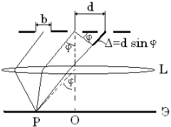
By consideration of spatial coherence the criterion enters the name as:
![]() ,
(4.13)
,
(4.13)
where φ is the angular size of a source, d is its linear size. At displacement along a wave surface emitted by a source the distance on which the phase varies no more than on π refers to as length( or radius) spatial coherence
![]() ~
~![]() .
(4.14)
.
(4.14)
For solar beams φ ~ 0,01rad, λ
~ 0,5 microns. Then ![]() =0,05
mm.
=0,05
mm.
 From
natural sources we have already considered a principle of supervision of
interference. We shall result an example of calculation of interference in thin
films.
From
natural sources we have already considered a principle of supervision of
interference. We shall result an example of calculation of interference in thin
films.
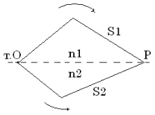
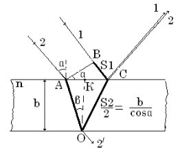
In figure 4.3 paths difference of beams 1 and 2 in a point C is equal:
![]() . (4.15)
. (4.15)
It is visible, that S1 = ВС; S2 = AO + OC;
КС = b* tg β;
Then ![]() and
and ![]() .
.
Figure 4.3
Let's substitute them in (4.15):
![]() .
.
Let's
make replacement ![]() . We
shall receive
. We
shall receive ![]() .
.
Having substituted last expression in Δ, we shall receive
![]() .
.
At
reflection of a beam 1 in a point with more dense environment the phase changes
on π, therefore on the right it is necessary to take away (or to add)![]() .
.
So a difference of a course:
![]() .
(4.16)
.
(4.16)
5 Lecture №5. Diffraction of waves
Lecture content: phenomenon of diffraction of light waves and methods of diffraction pattern calculation.
Lecture aim:
give students basic knowledge of:- the essence of light diffraction and condition of its supervision;
- principle of Huygence-Fresnel. Zones of Fresnel;
- examples of calculation of diffraction pattern;
- diffraction grating.
5.1 Phenomenon of light diffraction
The totality of phenomena observed in the propagation of light in the medium with sharp heterogeneities is named the diffraction. In particular, rounding of obstacles by light waves and penetration of light into area of a geometrical shadow is observed.
Condition of diffraction: d ~ λ.
Diffraction as well as interference is shown in redistribution of a light flow at imposing of coherent waves. Distinction is in next: at an interference the final number of light sources is considered, at diffraction light sources are located continuously.
The scheme of supervision of diffraction contains a source of light, an opaque barrier (a slit in a barrier) and the screen.
There are two kinds of diffraction: diffraction of Fresnel for spherical waves and diffraction of Fraunhofer for flat waves.
5.2 Principle of Huygence-Fresnel
Principle
of Huygence
explains a penetration of light into area of a shadow, but does not give data
about the amplitude of waves. According to principle of Huygence-Fresnel the
account of amplitudes and phases of secondary waves at their interference
allows to find amplitude of a resulting wave in any point. The amplitude of
oscillations is proportional dS and decreases with distance r and oscillation:
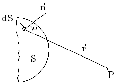
Figure 5.1
![]() (5.1)
(5.1)
сomes from each site dS of wave surface S into point Р and for all surface S we received
![]() (5.2)
(5.2)
The factor K(φ) = 1 at φ = 0; K(φ) = 0 at φ = π/2.
Calculation by the formula (5.2) is a very complicated problem but at the certain symmetry a definition of amplitude by a method of Fresnel zones is greatly simplified.
Essence of a method: The spherical wave propagates from a point source S of light. Wave surfaces are symmetric with respect to SP. Let's break a wave surface into ring zones of equal area so that distances up to point of supervision Р will differ from edges of each next zone on λ/2. Then oscillations in point Р from two next zones come in an antiphase and as amplitudes from the equal areas of a wave surface are considered identical then at even number of zones in point Р there will be a minimum of intensity (amplitude), and at odd number of zones - a maximum.
5.3 The method of Fresnel zones
The method of Fresnel zones has allowed explaining the law of rectilinear propagation of light on the basis of the wave theory. Then let's consider 3 examples:
An example 1: Diffraction of Fresnel from a round aperture.
Let on a way of a light wave there is an opaque screen with a round aperture of radius r0. For the given case underlying ratio is valid:
![]() .
(5.3)
.
(5.3)
Let's define from (5.3) number of open zones of Fresnel:
![]() .
(5.4)
.
(5.4)
Then we shall write down the expression for amplitude in point Р:
![]() ;
(5.5)
;
(5.5)
![]() .
(5.6)
.
(5.6)
Mark “minus” means that oscillations in P coming from adjacent zones are in antiphase.
![]() .
.
If m
is odd ![]() (maximum
I in the center). (5.7)
(maximum
I in the center). (5.7)
If m is even ![]() (minimum I in
the center). (5.8)
(minimum I in
the center). (5.8)
An example 2: Diffraction from a round opaque disk.
The first m zones are closed hence:
![]()
or
![]() .
(5.9)
.
(5.9)
We have always a maximum in the center.
All specified formulas are valid at small m.
5.4 The diffraction grating
 The
diffraction grating is a set of identical slits
spaced
at
equal distance from each other and separated by opaque intervals.
The
diffraction grating is a set of identical slits
spaced
at
equal distance from each other and separated by opaque intervals.
The period (or constant) of a grating is distance between the middle of the adjacent slits.
Intensity:
 .
.
Figure 5.2
Condition for minima for single slit and grating are identical:
![]() , k =
1,2,3… (5.10)
, k =
1,2,3… (5.10)
Condition for
main maxima: ![]() (5.11)
(5.11)
Condition for additional minima of a diffraction grating is:
![]() (5.12)
(5.12)
where ![]()
Their
number is equal (N-1) in intervals between the adjacent main
maxima. ![]() accepts
all integer values except for 0, N, 2N …
accepts
all integer values except for 0, N, 2N …
Number of main maxima:
![]() . (5.13)
. (5.13)
Intensity of main maxima grows proportionally to a square of number of slits:
![]() .
(5.14)
.
(5.14)
Position of the main maxima depends from λ. Red beams deviate more strongly than violet as against a dispersive spectrum. The diffraction grating works as the spectral device decomposing white light in a spectrum. The main parameters of the grating as a spectral device:
Angular
dispersion ![]() .
.
Linear
dispersion ![]() .
.
Resolution ![]()
6 Lecture №6. Polarization of light
Lecture content: phenomenon of polarization of light waves and its laws. Lecture aim:
give students basic knowledge of:
- the essence of light polarization;- the laws of Malus and Brewster.
6.1 Natural and polarized light
Light is a light
if the direction of light vector ![]() oscillations are ordered in a
certain way (for example, occur in a particular direction). In natural
(non-polarized) light, oscillations occur in different directions quickly and
randomly change each other.
oscillations are ordered in a
certain way (for example, occur in a particular direction). In natural
(non-polarized) light, oscillations occur in different directions quickly and
randomly change each other.
There are the following types of polarization states of light:
a) linear polarization;
b) elliptical polarization;
c) circular polarization (figure 6.1). In the latter two cases the light vector may be rotated either clockwise or counterclockwise. In all pictures light has the direction perpendicular to plane of figure.
Devices that allow obtaining linear -polarized light from natural light are called polarizers.
They pass
oscillations of vector ![]() in the plane called the plane
of polarization and don’t pass partially or completely in the perpendicular
plane.
in the plane called the plane
of polarization and don’t pass partially or completely in the perpendicular
plane.
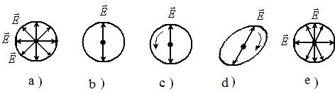
Figure 6.1
There is another type of polarized light: it is a partially polarized light, for which the concept of the degree of polarization is introduced:
![]() .
(6.1)
.
(6.1)
For example, for
a plane-polarized light ![]() and
and ![]() ; and for a
natural light
; and for a
natural light ![]() и
и ![]() .
.
Polarized light
is obtained by addition of two mutually perpendicular and coherent oscillations
![]() и
и ![]() :
:
 .
(6.2)
.
(6.2)
If the phase
difference ![]() is
equal to zero or π, we obtain:
is
equal to zero or π, we obtain:
![]() ,
(6.3)
,
(6.3)
that is plane-polarized
light. If ![]() then
(2) becomes the equation of the ellipse
then
(2) becomes the equation of the ellipse
 .
(6.4)
.
(6.4)
If ![]() from (4) we
obtain the equation of a circle:
from (4) we
obtain the equation of a circle:
![]() ,
(6.5)
,
(6.5)
where ![]() .
.
Equations (6.4)
and (6.5) correspond to the light polarized along an ellipse and a circle.
Cases ![]() and
and ![]() differ in the
direction of motion along an ellipse or a circle.
differ in the
direction of motion along an ellipse or a circle.
An oscillation
amplitude in a plane forming an angle ![]() with a plane of the polarizer
can be decomposed into two oscillations with amplitudes
with a plane of the polarizer
can be decomposed into two oscillations with amplitudes ![]() and
and ![]() , where
, where ![]() - the angle
between A and AY. The first oscillation passes through a polarizer
and the second will be delayed. The intensity of the wave is proportional to
the square of the amplitude. Then we can receive the Malus law for the
light wave intensity transmitted through the polarizer:
- the angle
between A and AY. The first oscillation passes through a polarizer
and the second will be delayed. The intensity of the wave is proportional to
the square of the amplitude. Then we can receive the Malus law for the
light wave intensity transmitted through the polarizer:
![]() . (6.6)
. (6.6)
6.2 Polarization at the reflection and refraction of light
Upon reflection from the conductive metal surface the elliptic polarized light is obtained. When light is incident at a certain angle on the boundary between two dielectrics reflected and refracted rays are partially polarized. The reflected light is dominated by oscillations perpendicular to the plane of incidence, in refracted light is dominated by parallel oscillations. The degree of polarization is dependent on the angle of incidence. At a certain angle satisfying the condition:
![]() , (6.7)
, (6.7)
where ![]() is the index of
refraction of the second medium with respect to the first medium. In this case
the reflected ray is completely polarized. It contains only oscillations
perpendicular to the plane of incidence. The refracted beam is partially
polarized, but has the greatest degree of polarization. Equation (6.7)
expresses the law of Brewster and the angle is called the Brewster
angle. Given the law of refraction it can be shown from Brewster's law that
the reflected and refracted rays are perpendicular. An explanation of the
polarization of the reflected and refracted rays can be specified on the basis
of the emission of light by atoms as the electric dipoles when in the fall of
light at the Brewster angle the direction of the reflected light coincides with
the axis of the dipole.
is the index of
refraction of the second medium with respect to the first medium. In this case
the reflected ray is completely polarized. It contains only oscillations
perpendicular to the plane of incidence. The refracted beam is partially
polarized, but has the greatest degree of polarization. Equation (6.7)
expresses the law of Brewster and the angle is called the Brewster
angle. Given the law of refraction it can be shown from Brewster's law that
the reflected and refracted rays are perpendicular. An explanation of the
polarization of the reflected and refracted rays can be specified on the basis
of the emission of light by atoms as the electric dipoles when in the fall of
light at the Brewster angle the direction of the reflected light coincides with
the axis of the dipole.
7 Lecture №7. Dispersion of light
Lectures content: phenomenon of light waves dispersion and its laws. Lecture aim:
give students basic knowledge of:
- the kinds and essence of light dispersion;
- the group velocity and its relation with phase velocity.
7.1 Normal and abnormal dispersion
The phenomena due to the substance refractive index dependence on wavelength of light wave are called dispersion of light. This dependence can be written by expression:
![]() , (7.1)
, (7.1)
where
![]() is
the wavelength of light wave.
is
the wavelength of light wave.
For all transparent colorless substances function (7.1) has dependence in visible part of spectrum shown in figure 7.1.
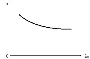 This
figure shows the phenomenon of normal dispersion when refractive index
decreases with increasing wavelength. If a substance absorbs a some rays
dispersion’s curve displays an anomaly in the absorption region and its
vicinity. In this interval of
This
figure shows the phenomenon of normal dispersion when refractive index
decreases with increasing wavelength. If a substance absorbs a some rays
dispersion’s curve displays an anomaly in the absorption region and its
vicinity. In this interval of ![]() dispersion of
substance
dispersion of
substance![]() is positive and dependence (7.l) is called the abnormal dispersion.
is positive and dependence (7.l) is called the abnormal dispersion.
Figure 7.1
7.2 Group velocity and its relation with phase velocity
The superposition of waves of slightly different frequency is called a wave packet or the group of waves. Analytical expression for a group of waves has the form:
 (7.2)
(7.2)
if following condition is satisfied:
![]() .
.
For a group of waves the following relation holds
![]() .
(7.3)
.
(7.3)
Where
![]() is
spread of x values and
is
spread of x values and ![]() is spread of values of wave number.
is spread of values of wave number.
If
dispersion is absent in medium all plane waves forming a wave packet propagate
with same phase velocity![]() . It is clear that the velocity
of moving packet also equals
. It is clear that the velocity
of moving packet also equals![]() . If dispersion in medium is
small a moving packet does not run over time. In this case the center of wave
packet (the point with maximal value of E) moves with group velocity
. If dispersion in medium is
small a moving packet does not run over time. In this case the center of wave
packet (the point with maximal value of E) moves with group velocity![]() . It is the
velocity of wave energy propagation. If the medium has dispersion in case when
. It is the
velocity of wave energy propagation. If the medium has dispersion in case when ![]() we have
we have ![]() and in case
when
and in case
when ![]() the
group velocity is more than phase velocity, i.e.
the
group velocity is more than phase velocity, i.e. ![]() .
.
The phase velocity is defined as velocity of propagation of phase of wave or
![]() .
(7.4)
.
(7.4)
The group velocity is defined by expression:
![]() .
(7.5)
.
(7.5)
Let’s set the
relationship between these velocities. Since ![]() we can write
(7.5) in following form:
we can write
(7.5) in following form:
![]() (7.6)
(7.6)
and then
![]() .
.
From
ratio ![]() it
is follows that
it
is follows that
![]() .
.
Accordingly
![]() .
.
Substitute the
right side of last expression for ![]() we shall receive
we shall receive
![]() .
(7.7)
.
(7.7)
This
formula shows that depending on the sign of ![]() the group velocity
the group velocity ![]() may be as low
as or greater than phase velocity
may be as low
as or greater than phase velocity ![]() . If
. If ![]() , i.e. in the
absence of dispersion the group velocity has the same value with the phase.
, i.e. in the
absence of dispersion the group velocity has the same value with the phase.
8 Lecture №8. Thermal radiation
Lectures content: laws of thermal radiation, radiation of absolutely black body, Planck's law№
Lecture aim:
give students basic knowledge of:
- characteristics and basic laws of thermal radiation;
- a problem of radiation of absolutely black body;
- a hypothesis and Planck's law.
We have considered the phenomena of wave optics. Now we shall consider corpuscular properties of electromagnetic radiation. We shall begin with thermal radiation as one of its kinds.
8.1 Characteristics and basic laws of thermal radiation
Emission of electromagnetic waves due to internal energy of bodies is called thermal radiation. All other kinds of radiation refer to luminescence. Only thermal radiation can be equilibrium and it occurs at any temperature above absolute zero.
Power
luminosity of a body R and
emissive ability of a body ![]() are
connected among themselves by a ratio
are
connected among themselves by a ratio
 . (8.1)
Let
the flow of radiant energy falling on an element of the area, is equal ![]() , and
, and ![]() the part of a
stream absorbed by a body. Dimensionless quantity
the part of a
stream absorbed by a body. Dimensionless quantity
![]() ,
(8.2)
,
(8.2)
refers to ability
of a body. For absolutely black body![]() , if
, if ![]() the
body refers to grey bodies.
the
body refers to grey bodies.
а) the Kirchhoff's law states that the ratio of emissive ability of a body to its absorption ability does not depend by nature of bodies, it is for all bodies the same (universal) function of frequency (length of a wave) and temperatures:
Universal function f (w, Т) is испускательная ability of absolutely black body.
![]() (8.3)
(8.3)
or  .
. ![]() (8.4)
(8.4)
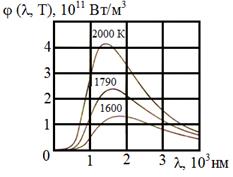
Absolutely black bodies do not exist naturally. However it is possible to create his (its) model, i.e. almost closed cavity supplied with a small aperture, and radiation, penetrated inside, testing repeated reflections, practically it is completely absorbed. According to the Kirchhoff's law emissivity ability of model is very close to f (w, Т), where Т - temperature of walls of a cavity. Then the aperture is left with the radiation close on spectral structure to radiation of absolutely black body.
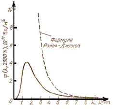
Results
of experiences on research of behavior of function ![]() are resulted in
figure 8.1.
are resulted in
figure 8.1. ![]()
 b) Stefan–Boltzmann
law connects
power luminosity of absolutely black body with its absolute temperature
b) Stefan–Boltzmann
law connects
power luminosity of absolutely black body with its absolute temperature
 , (8.5)
where s - Stefan–Boltzmann constant.
c) the
law of displacement the Fault connects
absolute temperature and length of a wave ![]() on which it is necessary a
maximum of function
on which it is necessary a
maximum of function ![]()
Figure
8.1 ![]() , (8.6)
, (8.6)
where b - a
constant equal b = of 2,9010 ![]() m.
m.
d) the second law the Fault gives dependence of the maximal spectral density of power luminosity of a black body on temperature:
![]() , (8.7)
, (8.7)
where constant ![]() .
.
8.2 Problems of radiation of absolutely black body
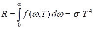
Rayleigh–Jeans law received on the classical theory looks as follows:
![]() . (8.8)
. (8.8)
This formula will well be coordinated to experimental data only at the big lengths of waves and sharply misses experience for small lengths of waves (figure 8.2). Substitution of the formula (8.10) in (8.6) gives for equilibrium density of energy u (T) indefinitely great value. This result which has received the name of ultra-violet accident, also contradicts experience.
Balance between radiation and a radiating body is established at final values of f(w, T).
Figure 8.2
8.3 A quantum hypothesis and formula of Planck
In
1900 Planck managed to find a kind of the function ![]() corresponding to
experimental data. For this purpose it(he) has put forward a hypothesis, that
electromagnetic radiation is let out as separate portions of energy-
corresponding to
experimental data. For this purpose it(he) has put forward a hypothesis, that
electromagnetic radiation is let out as separate portions of energy-
Quantum which size is proportional to frequency of radiation:
![]() .
(8.9)
.
(8.9)
Here h or ![]() - Planck's
constant.
- Planck's
constant.
It is possible to show, that average energy of radiation of frequency w is equal
![]() . (8.10)
. (8.10)
Then 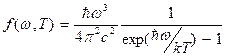 .
(8.11)
.
(8.11)
Planck's formula (8.11) gives the exhaustive description of equilibrium thermal radiation.
9 Lecture №9. Corpuscular properties of electromagnetic radiation
Lecture content: Corpuscular-wave dualism of electromagnetic radiation and its applications.
Lecture aim:
give students basic knowledge of:
- corpuscular-wave dualism of electromagnetic radiation. Photons, experiment of Bothe;
- Compton scattering.
9.1 Experiment of the Bothe. Photons. Energy and a pulse of a photon
Except for two hypotheses (Planck for thermal radiation and Einstein for a external photoelectric effect) Einstein had put forward next (third) hypothesis about propagation of light in space as discrete particles (This particle was quantum, later its name is photon). Experience the Bothe (1926) is an experimental confirmation of this hypothesis.
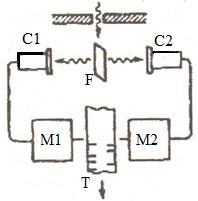 In
this experiment a thin metallic foil F placed between two gas-discharge counters.
Foil exposed to a weak beam of X-rays and itself became a secondary X-ray
source. The number of photons emitted by the foil was small due to the low
intensity of the initial source. Counters C1 and C2 are triggered by hit of
X-rays in them and powered mechanisms M1 and M2 made marks on the moving tape T.
From the wave theory it follows that counters should be triggered at the same
time at a uniform radiation in all directions but in the experiment the marks on
the tape are not the same.
In
this experiment a thin metallic foil F placed between two gas-discharge counters.
Foil exposed to a weak beam of X-rays and itself became a secondary X-ray
source. The number of photons emitted by the foil was small due to the low
intensity of the initial source. Counters C1 and C2 are triggered by hit of
X-rays in them and powered mechanisms M1 and M2 made marks on the moving tape T.
From the wave theory it follows that counters should be triggered at the same
time at a uniform radiation in all directions but in the experiment the marks on
the tape are not the same.
Thus the experience the Bothe confirms an existence of photons.
Figure 9.1
Energy of photon: ![]() . (9.1)
. (9.1)
Pulse of photon:
![]() . (9.2)
. (9.2)
The rest mass equals 0.
The
photon always goes with a speed ![]()
9.2 Corpuscular-wave duality (CWD)
Under the wave theory light exposure Е ~ А2 and under the corpuscular theory it ~ density of a flow of photons, i.e. А2 ~ density of a flow. The carrier of energy and a pulse is a photon, А2 gives a probability of hit of a photon in the given point. More accurate information – it is the probability of detection of a photon in volume dV containing the considered point and it is equal
![]() . (9.3)
. (9.3)
Conclusion of
the given consideration: Distribution of photons on a surface has a statistical
property. Observable uniformity of illumination is caused by the big density of
a flow of photons [I ~ 1013 photons / (sm2.sec)].
Relative fluctuation ~ ![]() . It is a very
small quantity and we see the uniform illumination of surface.
. It is a very
small quantity and we see the uniform illumination of surface.
9.3 Compton scattering
In 1923 A. Compton investigates a scattering of monochromatic X-rays by various substances has found out
that absent-minded beams alongside with radiation of initial length of a wave
fluctuation ![]() contain
also beams of the greater length
contain
also beams of the greater length ![]() of a wave. Appeared
that
of a wave. Appeared
that
![]() . (9.4)
. (9.4)
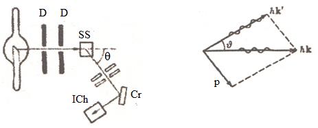
Figure 9.2 Figure 9.3
![]() is
the angle of scattering, i.e. a difference
is
the angle of scattering, i.e. a difference ![]() does not depend
on a nature of substance and a wave length
does not depend
on a nature of substance and a wave length ![]() . The circuit of
experience is shown on figure 9.2 (D –diaphragm, SS – scattering substance, Cr
– crystal and ICh – ionization chamber).
. The circuit of
experience is shown on figure 9.2 (D –diaphragm, SS – scattering substance, Cr
– crystal and ICh – ionization chamber).
Effect
of Compton speaks having presented scatter as process
of elastic collision of x-ray photons with almost free electrons. If the
photon with energy ![]() Falls on
originally based electron and a pulse
Falls on
originally based electron and a pulse ![]() (figure 9.3)
using laws of conservation of energy and a pulse it is possible to receive the
formula (9.4),
where
(figure 9.3)
using laws of conservation of energy and a pulse it is possible to receive the
formula (9.4),
where
![]() (9.5)
(9.5)
![]() is named as
Compton/s length of a wave for electron.
is named as
Compton/s length of a wave for electron.
![]() .
.
10 Lecture №10. Wave properties of microparticles
Lecture content: hypothesis of de-Broglie. Wave properties of substance and microparticles.
Lecture aim:
- to comprehend a hypothesis de Broglie and wave properties of substance;
-to study the principle of a ban of Pauli and Schrödinger's equation.
10.1 Hypothesis of de-Broglie. Wave properties of substance
Insufficiency of Bohr’s theory indicated the need of revision of quantum theory bases and ideas of the microparticles nature. There was a question of that representation of an electron in the form of the small mechanical particle characterized by certain coordinates and a certain speed is doubtful.
As a result of deepening of light nature ideas it became clear that in the optical phenomena a peculiar dualism is found. Assuming that substance particles along with corpuscular properties have as well wave properties de Broil put out hypothesis that substance particles should also have wave properties. He used the well-known formulas of wave and particle properties relation for photons.
The photon possesses energy
![]() and
an impulse
and
an impulse ![]() .
(10.1)
.
(10.1)
In principle de-Broglie connected the movement of non-relativistic electron or any other microparticle with wave process which wavelength is equal to
 and frequency
  (10.2)
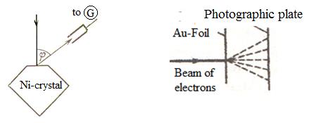
Figure 10.1 Figure 10.2
For the first time Davisson and Germer confirmed the hypothesis of de Broglie in 1927. The narrow beam of monoenergetic electrons went to a Ni-monocrystal surface. The reflected electrons were caught by the cylindrical electrode attached to a galvanometer G (figure 10.1). Intensity of the reflected beam was estimated on current flowing through a galvanometer. Speed of electrons and an angle φ varied. Experimental results for the wavelength of the electron beam obtained by the Bragg formula coincided with the wavelength calculated by the formula (10.2) for λ. This was a convincing proof of this hypothesis.
G. P. Thomson (1927) and irrespective of him P. S. Tartakovsky received a diffraction picture when passing an electron beam through a metal foil.
Experience was carried out as follows. The beam of the electrons accelerated by a potential difference about several tens kilovolts passed through a thin metal foil and got on a photographic plate. The electron at blow about a photographic plate has on it the same effect as well as a photon. Received in such a way a gold gram of electrons it is compared with the roentgenogram of aluminum received in similar conditions.
10.2 Properties of microparticles
Elementary particles (electrons, protons, neutrons, photons and other simple particles) and also more complex particles consisting of small number of elementary particles (molecules, atoms, and atomic nuclei) are the microparticles. Any micro-object represents microparticle having as the properties of particle so the properties of wave. In other words, they have wave-particle duality.
However, they are neither true particles nor true waves because unlike the first (particles) they may not have the path in contrast to the second (waves) are not divided, so is a whole.
The originality of the properties of microparticles is shown in the following thought experiment. If you pass parallel beam of monochromatic electrons through two narrow slits and register a picture on the photographic plate you observe the phenomenon of electron diffraction which proves the participation of both slits in the passage of each electron although the electron is an indivisible whole.
This implies that the micro world objects have the qualitatively new properties have no analogues in our macrocosm.
11 Lecture №11. Elements of quantum mechanics
Lecture content: principle of uncertainty of Heisenberg. Schrödinger's equation and its applications.
Lecture aim: to give students basic knowledge about:
- principle of uncertainty of Heisenberg as the precision with which certain pairs of physical properties of a particle can be known;
- Schrödinger's equation as the basic equation which describes how the quantum state of a quantum system changes with time.
11.1 Principle of Heisenberg uncertainty
The statement about that product of values of two conjugate variables cannot be in the order of size less constant of Planck, is called as the principle of uncertainty of Heisenberg.
If
there are some (many) identical copies of system in this state, the measured
values of coordinate and an impulse will submit to a certain distribution of
probability - it is a fundamental postulate of quantum mechanics. Measuring the
size of a mean square deviation ![]() of coordinate
and a mean square deviation
of coordinate
and a mean square deviation ![]() of an impulse,
we will find that:
of an impulse,
we will find that:
![]() ,
(11.1)
,
(11.1)
where ħ - the given constant of Planck.
Let's
note that this inequality gives some opportunities — the state can be such
that ![]() can be measured
with high precision, but then
can be measured
with high precision, but then ![]() will be known
only approximately, or on the contrary
will be known
only approximately, or on the contrary ![]() can be defined
precisely, while
can be defined
precisely, while ![]() — no. In all
other states x and p c
— no. In all
other states x and p c![]() be also measured
with "reasonable" (but not random high) accuracy.
be also measured
with "reasonable" (but not random high) accuracy.
Following relation of uncertainty between energy and time:
![]() (11.2)
(11.2)
where
![]() is an
uncertainty of change of energy of system;
is an
uncertainty of change of energy of system;
![]() -
measurement duration.
-
measurement duration.
Pauli's principle (the principle of a ban) — For all fermions fairly the statement: in system in the same quantum state there cannot be more than one fermion.
The steady quantum state of an electron in atom is characterized by four quantum numbers: main thing p (p = 1, 2, 3, 4), orbital / (/= 0,1,2..., and - 1), to magnetic t (-/,-1,0,1, +/), spin s (s = ±1/2).
Pauli's principle: in atom each electron possesses the set of quantum numbers other than a set of these numbers for any other electron.
11.2 Schrödinger's equation. Wave function
Schrödinger's equation in quantum mechanics as well as the second law of Newton in classical physics, is not output, and is postulated:
 , (11.3)
where m – the mass of a particle;
i – imaginary unit;
Ñ2– Laplace's operator;
U - potential energy of a particle in a force field in which it moves;
Ψ – required wave function.
If the force field in which the particle moves is permanent function U(x,y,z) does not depend obviously on time and has as it was already noted a meaning of potential energy. In this case the solution of the equation of Schrödinger breaks up to two multipliers one of which depends only on coordinates, another — only on time:
![]() .
.
The differential equation defining function ψ becomes as
 . (11.4)
or
![]() . (11.4´)
. (11.4´)
This is basic equation of non-relativistic quantum mechanics.
![]() is complex
function (psi – function) coordinates and time characterizing the state of
microparticles.
is complex
function (psi – function) coordinates and time characterizing the state of
microparticles.
According to Born (1926) square function module determines the probability dP that a particle will be detected within the volume dV
![]() .
.
А - the factor of proportionality, for the psi-function the following condition normalization condition is carried out:
![]() .
.
Psi - function must be unambiguous, continuous and finite, moreover, it should have continuous and finite derivative - standard conditions.
11.3 A particle in rectangular infinitely deep potential pit
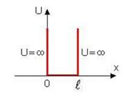 Let
the particle goes along an axis X in infinitely deep potential pit. In this
case Potential energy is equal to zero inside a pit (figure 11.1). Because of
infinite height of potential walls the particle cannot get for limits of a
potential pit hence inside and outside of a pit function equals 0 and we have
border conditions:
Let
the particle goes along an axis X in infinitely deep potential pit. In this
case Potential energy is equal to zero inside a pit (figure 11.1). Because of
infinite height of potential walls the particle cannot get for limits of a
potential pit hence inside and outside of a pit function equals 0 and we have
border conditions: ![]() .
.
Figure 11.1
We use stationary equation of Schrödinger
![]() . (11.5)
. (11.5)
In the field of 0 <x <l Schrödinger's equation looks like:
![]() (11.6)
(11.6)
Let's
designate: ![]() . (11.7)
. (11.7)
Then the
equation will become: ![]() . (11.8)
. (11.8)
The solution
of (11.8): ![]() . (11.9)
. (11.9)
We
use (11.5) for definition k and![]() . From
. From ![]() we receive
we receive ![]() whence
whence![]() .
.
From ![]() we have
we have ![]() and
and ![]() , (11.10)
, (11.10)
where
![]() and
it is a quantum number.
and
it is a quantum number.
Let's substitute (11.10) in (11.7) and we shall find own values of energy:
![]() (11.11)
(11.11)
The spectrum of energy appeared discrete.
Let's estimate distance between the next power levels:
 .
.
For molecules (m ~ 10-26 kg) of gas in a vessel with the sizes l ~ 0,1 m calculation gives that ΔЕn ~10-39 n, J≈ 10-20 n, eV. So densely located energy levels form practically continuous spectrum of energy so quantization of energy will not affect on character of motion of molecules. But for electron the size of atom (l ~ 1010 m) leads to other result: ΔЕn ~102 n, eV. Here a step-type form of levels is appreciable.
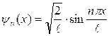
Wave function looks like:
![]() . (11.12)
. (11.12)
Then we use a condition of normalization:
 .
.
On
borders function = 0 therefore integral equals an average value of the
function increased for length of an interval ℓ, i.e. ![]() , whence
, whence ![]() and
and
 . (11.13)
Consider the graphs of wave function and probability density on coordinate x.
Figure 11.2
Now
consider a principle of conformity of Bohr. Let’s define an influence of
quantum number n on character of an arrangement of levels. From (11.11) and
next formula for ![]() we have
we have ![]() .
.
This
expression shows: with growth n ![]() decreases, i.e. relative
approach of levels takes a place. In 1923 Nils Bohr had formulated a
principle of conformity:
decreases, i.e. relative
approach of levels takes a place. In 1923 Nils Bohr had formulated a
principle of conformity:
At the big quantum numbers results and conclusions of quantum mechanics should correspond to classical conclusions and results.
11.3 Passage of a particle through a potential barrier
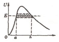
Let's consider 2 cases: classical and quantum. In quantum case the tunnel effect is possible. The factor of a transparency of a barrier is equal to:
![]() .
(11.14)
.
(11.14)
Figure 11.3
оr
![]() . (11.15)
. (11.15)
It gives
a probability of passage of waves de Broglie through
a potential barrier. By analogy to optics the factor of reflection ![]() is entered
also.
is entered
also.
For a rectangular barrier
![]() .
(11.16)
.
(11.16)
The tunnel effect takes place when D is not too small, i.e. the exponent is close to 1. It is possible at ℓ about the nuclear sizes.
Example: U-E ≈ 10 eV, me ≈ 10-30 kg, ℓ ≈ 10-10 m, a degree ≈ 1 and D ≈ 1/e.
In classical
case particle doesn’t always pass through barrier if the particle energy E is
less than the height U of barrier and always passes if ![]()
12 Lecture №12. Atom of hydrogen
Lecture content: atom of hydrogen and its significance.
Lecture aim: to give students basic knowledge about:
- Bohr model of atom of hydrogen;
- significance in quantum mechanics and quantum field theory.
Swiss physicist Balmer (1885) defines a cyclic frequency of light:
![]() (12.1)
(12.1)
where R = 2,07.1016 c-1. Generalized formula of Balmer gives a cyclic frequency of other spectral series of hydrogen atom radiation:
![]() ,
(12.2)
,
(12.2)
where
![]()
The solution of quantum mechanics problem for hydrogen atom
Potential energy of interaction of an electron with the nucleus possessing Ze charge (for atom of hydrogen Z = 1),
 ,
(12.3)
,
(12.3)
where r - distance between an electron and a nucleus.
Equation of Schrödinger:
 ,
(12.4)
,
(12.4)
The solution of this equation for standard conditions:
 .
(12.5)
.
(12.5)
At ![]() (the basic state
of atom):
(the basic state
of atom): ![]() .
.
Paul in whom the
electron moves, is central symmetric. Therefore it is necessary to use
spherical system
of
coordinates: r, ![]()
Own functions:
![]() .
(12.6)
.
(12.6)
At given n: ℓ = 0,1,2, …, n-1.
At given ℓ: m = - ℓ, - ℓ +1,-1, 0, 1, … ℓ-1, ℓ ; i.e. (2 ℓ + 1) values.
Energy
depends only from n. Hence to everyone ![]() there correspond some own
functions
there correspond some own
functions ![]() with
different ℓ and m for given n. Different states with identical energy
refer to degenerated.
with
different ℓ and m for given n. Different states with identical energy
refer to degenerated.
Frequency
rate of degeneration ![]() . (12.7)
. (12.7)
Possible states of electrons:
1s
2s 2p
3s 3p 3d
4s 4p 4d 4f, etc.
Rule
of selection:
![]() .
.
To show the circuit of transitions in atom of hydrogen.
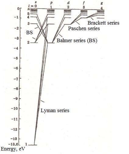
Figure 12.1
Spatial quantization
In
quantum mechanics it is proved that to Schrödinger's equation satisfy own
functions ![]() ,
determined by three quantum numbers: main n, orbital l, and magnetic
,
determined by three quantum numbers: main n, orbital l, and magnetic ![]() .
.
The main quantum number n determines power levels of an electron in atom and can accept any integer values, since unit: n = 1,2,3, …
Follows from the solution of the equation of Schrödinger that the impulse moment (the mechanical orbital moment) of an electron is quantized:
![]() (12.8)
(12.8)
where l – orbital quantum number which at the set n accepts values
l = 0,1, …, (n – 1) (12.9)
i.e. all n of values, also defines the electron impulse moment in atom.
Follows from the
solution of the equation of Schrödinger also that a vector ![]() the moment of
an impulse of an electron can have only such orientations in space, at which
its projection
the moment of
an impulse of an electron can have only such orientations in space, at which
its projection ![]() on
the direction z of an external magnetic field accepts quantized
values, multiple
on
the direction z of an external magnetic field accepts quantized
values, multiple ![]() :
:
![]() ,
(12.10)
,
(12.10)
where ![]() - magnetic
quantum number which at the set l can accept values
- magnetic
quantum number which at the set l can accept values
![]() i.e. all 2l + 1
values.
i.e. all 2l + 1
values.
Thus, magnetic
quantum number ![]() defines an
electron impulse
moment
projection
to
the set direction, and the electron impulse moment vector
in atom can have in space 2l
+
1 orientations. Number of various states corresponding to this n,
equally
defines an
electron impulse
moment
projection
to
the set direction, and the electron impulse moment vector
in atom can have in space 2l
+
1 orientations. Number of various states corresponding to this n,
equally
![]() (12.11)
(12.11)
Quantum numbers n and l characterize the size and a form of an electronic cloud in space.
Quantum numbers n, l, and ![]() allow
describing more fully the range of emission (absorption) of
atom of hydrogen received in
Bohr's theory.
allow
describing more fully the range of emission (absorption) of
atom of hydrogen received in
Bohr's theory.
In quantum mechanics the rules of selection limiting number of possible transitions of the electrons in atom connected with emission and absorption of light are introduced:
1) change of
orbital quantum number ![]() meets a condition
meets a condition
![]() (12.12)
(12.12)
2) change of
magnetic quantum number ![]() meets a condition
meets a condition
![]() (12.13)
(12.13)
It is entered also electron backs – own moment of an impulse.
13 Lecture №13. Elements of quantum statistics
Lecture content: elements of quantum statistics and their application to main problems of quantum physics.
Lecture aim:
give students basic knowledge of:
-concept about quantum statistics of Bose-Einstein and Fermi - Dirac. Bosons and fermions;
- degenerated electronic gas in metals. Fermi's level;
- electrical conductivity of metals.
13.1 Concept about quantum statistics of Bose-Einstein and Fermi - Dirac. Bosons and fermions
In quantum statistics the systems consisting of huge number of particles, are investigated with the help of laws of quantum mechanics in which basis lay corpuscular - wave dualism of particles of substance and a principle of indistinguishability of identical particles. Last means, that all identical particles (for example, electrons in metal) are indiscernible from each other.
In
quantum statistics, a problem about distribution of particles on cells
of phase space (six-measured space of coordinates and speeds) which element is
equal ![]() and also a
problem of definition of average values of the physical sizes describing a
macroscopic condition of system are considered. To a condition of a particle in
phase space in view of a ratio of uncertainties of
Heisenberg
there corresponds(meets) not a point, and a cell of phase volume h3,
where h - Planck's constant.
and also a
problem of definition of average values of the physical sizes describing a
macroscopic condition of system are considered. To a condition of a particle in
phase space in view of a ratio of uncertainties of
Heisenberg
there corresponds(meets) not a point, and a cell of phase volume h3,
where h - Planck's constant.
Particles which number equals ΔNi in volume ΔGi can in the various ways to be distributed between Δgi conditions with energy Ei. Then the number of quantum states in volume ΔGi with energy from Ei up to Ei + ΔEi equals
![]() . (13.1)
. (13.1)
Average value of any function is defined with the help of function of distribution which allows finding probability of the given condition of system also.
In
quantum mechanics distinguish two kinds of particles: bosons are
particles with the integer or zero spin (in
terms of![]() ) for which Pauli's principle
doesn’t use and submitting to Bose-Einstein's distribution
(for example, some nuclei, photons, phonons) and fermions particles with
half-integer
spin (electrons,
protons, neutrons, etc.). The last are described by Fermi - Dirac quantum
statistics and submit to Pauli's principle according to which in each quantum
condition there can be only one particle. Function of distribution of Bose-Einstein fB
expresses average "density of boson population" in states with the
given energy or their average number in one condition:
) for which Pauli's principle
doesn’t use and submitting to Bose-Einstein's distribution
(for example, some nuclei, photons, phonons) and fermions particles with
half-integer
spin (electrons,
protons, neutrons, etc.). The last are described by Fermi - Dirac quantum
statistics and submit to Pauli's principle according to which in each quantum
condition there can be only one particle. Function of distribution of Bose-Einstein fB
expresses average "density of boson population" in states with the
given energy or their average number in one condition:
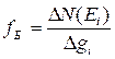 ,
,
Where
![]() - number of particles with
energy in an interval from Ei up to Ei + ΔEi;
- number of particles with
energy in an interval from Ei up to Ei + ΔEi;
![]() -
number of quantum conditions in this energy interval.
-
number of quantum conditions in this energy interval.
Distribution of bosons on energy turns out from initial distribution of Gibbs under condition of conservation of energy E in system and number of particles N:
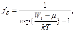 (13.2)
where k is Boltzmann¢s constant Т - thermodynamic temperature;
μ - the chemical potential equal to work made in isobaric-isothermal conditions at increase in number of particles in system on unit.
μ ≤ 0, differently the average number of bosons in the given condition becomes negative that is deprived sense.
Function of distribution of Fermi - Dirac is defined similarly:
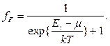 (13.3)
Here μ as against (2) can be positive.
In classical (Maxwell-Boltzmann) and quantum statistics of interpretive as an average of particles in one state it is possible to express functions of distribution by the uniform formula:
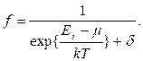 (13.4)
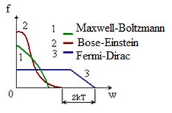 For
distribution Maxwell-Boltzmann's δ = 0 and
μ = 0, for Bose-Einstein's distribution δ
=-1 and for Fermi - Dirac's distribution δ = +1. All three distributions
are shown on figure 13.1.
For
distribution Maxwell-Boltzmann's δ = 0 and
μ = 0, for Bose-Einstein's distribution δ
=-1 and for Fermi - Dirac's distribution δ = +1. All three distributions
are shown on figure 13.1.
The system of particles refers to degenerate if its properties are described by quantum laws. Degeneration becomes essential for bose- or fermi-gases at low temperatures and the big density.
Figure 13.1
The
quantity![]() is
named the parameter of degeneration. At A
<<1 (small degeneration) in (4) it is possible to neglect size
δ and quantum functions of distribution pass in classical. The parameter
and is defined from a condition of preservation of the general number of
particles:
is
named the parameter of degeneration. At A
<<1 (small degeneration) in (4) it is possible to neglect size
δ and quantum functions of distribution pass in classical. The parameter
and is defined from a condition of preservation of the general number of
particles:
 (13.5)
where n - concentration of particles;
m - mass of a particle;
Т – temperature;
k - constant of Boltzmann;
h - Planck's constant.
Example of generated gas are electrons in metal which do not submit to classical statistics of Maxwell-Boltzmann.
13.2 Fermi's level
Electrons in metal behave as a molecule of ideal gas (electronic gas). They are in a three-dimensional potential hole, their energy quantized. Distribution on power levels submits Fermi - Dirac to distribution. The average electrons at level Еi is equal:
 , (13.6)
where EF is a Fermi's energy or level; EF > 0.
The number of quantum conditions электронов in unit of volume of metal in an interval энергий from E up to E + dE is equal:
 (13.7)
with
the account p2
= 2mE, 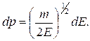
The number of electrons in unit of volume of metal for энергий from E up to E + dE is equal:
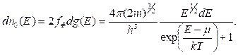 (13.8)
The factor 2 takes into account, that electrons submit to Pauli's principle.
So the law of distribution of electrons on energy is received.
At absolute zero (Т = 0 К) at E < μ where μ - chemical potential, we have fF → 1 and at E > μ0 fF → 0. The schedule of function of distribution of Fermi - Dirac fF at Т = 0 K is shown on figure 13.1. Clearly that μ represents the maximal energy электронов. It refers to Fermi's energy: μ = EF. The best level occupied by electrons in metal refers to Fermi's level.
The law of distribution of electrons in metal at Т = 0 looks like conductivity:
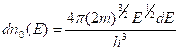 .
(13.9)
.
(13.9)
The general number electrons in unit of volume of metal equally:
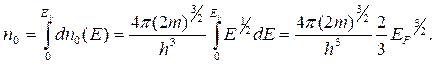 (13.10)
From here it is possible to define Fermi's energy
 (13.11)
And average energy of electron at Т = 0 K:
 (13.12)
Having taken concentration n0 = 6.1028 m-3 and corresponding values of constants, we shall receive <E> = 9.10-19 J = 5,4 eV.
13.3 Electrical conductivity of metals
According to the quantum theory a specific electric conductivity of metal is equal to expression
 , (13.13)
reminding the
classical formula but having the different physical contents. Here ![]() is an average
length of free run электрона with
the energy equal to energy of Fermi, and
is an average
length of free run электрона with
the energy equal to energy of Fermi, and ![]() is
an average speed of thermal movement such electron. The formula (13) yields the
results corresponding to the skilled data. Within the framework of the quantum
theory it is possible to explain it is abnormal great values of average length
of electrons free run in the metal exceeding the lattice period in hundreds times,
and also dependence σ ~ 1/T: the quantity
is
an average speed of thermal movement such electron. The formula (13) yields the
results corresponding to the skilled data. Within the framework of the quantum
theory it is possible to explain it is abnormal great values of average length
of electrons free run in the metal exceeding the lattice period in hundreds times,
and also dependence σ ~ 1/T: the quantity ![]() is defined by
expression
is defined by
expression
![]() ,
,
where Е is the module of Yang and d is the period of a lattice then
 , (13.14)
I.e.
σ ~ 1/T, whereas under the classical theory σ ~![]() .
.
14 Lecture №14. Zone theory of solids
Lecture content: main elements of zone theory of solids.
Lecture aim:
give students basic knowledge of:
- energy zones in crystals;
- semiconductors.
According to the zone theory the periodic electric field existing in the solids essentially changes energy conditions for electrons. Instead of characteristic for isolated atom of a level in a crystal, containing N cooperating atoms, the energy zones containing N of levels, shared by an interval about 10-23 эВ, are formed. Such allowed energy zones are shared by the forbidden zones (figure 14.1).
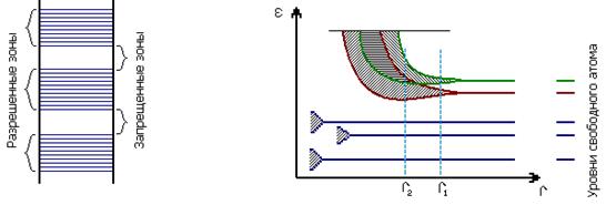
Figure 14.1 Figure 14.2
In figure 14.2 splitting levels as function of distance r between atoms is shown. Levels of valent electrons and overlying not occupied by electrons levels are appreciably split only. At distance such as r1 between zones there is a forbidden zone, at distance such as r2 there is an overlapping of the next zones.
Existence of energy zones allows explaining existence of metals, semiconductors and dielectrics. The allowed zone which has arisen from a level valent of electrons in the basic condition of atom is named a valent zone. Depending on a degree of filling of this zone three cases are possible:
а) this zone is filled by electrons not completely. The given crystal is metal.
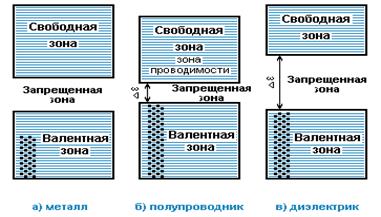
Figure 14.3
The same will be at overlapping of next allowed zones. в) the valent zone is filled completely and separated from the nearest allowed zone (a zone of conductivity) by small width of the forbidden zone ΔЕ (about the tenth shares of eV in FZ). Such crystal is the semiconductor;
b) if the width ΔЕ is great (over 5 eV), a crystal is a dielectrics.
2. Semiconductors.
Semiconductors (fig.4) are substances which specific resistance changes in a wide interval from 10-5 up to 108 Оhm.m and very quickly decreases with growth of temperature. Such semiconductors, as Si and Ge, are most widely applied. Distinguish intrinsic and impurity semiconductors.
Figure 14.4
Chemically pure semiconductors have the intrinsic conductivity. In them at Т = 0К all levels of valent zone (VZ) are filled by electrons. The electric field cannot throw them from valent conductivity into the zone of conductivity (ZC), therefore intrinsic semiconductors at Т = 0К behaves as dielectrics. At Т > 0 K as a result of thermal generation the part of electrons passes from top levels VZ to bottom levels ZC. Owing to formation of vacant levels in VZ the behaviour of electrons can be submitted as movement positively charged quasi-particles, named by holes.
Distribution of electrons on levels of VZ and ZC submits to Fermi - Dirac distribution. In intrinsic semiconductors value of a level of Fermi is equal
 .
(14.1)
.
(14.1)
where ΔЕ is the width of the forbidden zone; mH* and mE* are effective masses of a hole and electron in ZC. Usually the second item is small and EF = ΔE/2.
Electrical conductivity of intrinsic semiconductors depends on temperature under the following law
![]() ,
(14.2)
,
(14.2)
where ΔЕ is width of FZ, σ0 is a constant.
Having temperature dependence ln σ from 1/T, it is possible to define under the schedule width of the forbidden zone of the semiconductor ΔЕ.
Impurity conductivity are shared on electronic (or n-type) and hole (р-type) conductivity. For reception of the semiconductor of n-type (for example, silicon (Si) is an element of IY group) a donor impurity enter, i.e. element of Y group (phosphorus, arsenic, etc.). An atom Si has on the structure of 4 next atoms with which, giving on one electron forms covalent connections. The fifth electron of an atom of an impurity remains superfluous. Energy levels for such electrons settle down below a bottom of ZC, translation electrons in which needs small energy (for As in Si ΔED = 0,054 eV) received for example at thermal excitation. At replacement of atom Si by trivalent atom of accepted impurity (B, Al, etc.) There is a lack of one electron for formation of sated covalent connections. Missing electron can be borrowed from next atom Si at which appears thus a positive hole. Consecutive filling of holes by next electrons is equivalent to movement of holes and leads to conductivity of the semiconductor. The accepted levels arise in FZ the semiconductor above ceiling VZ (for In in Si ΔEA = 0,08 eV), transition of electrons from VZ on accepted levels leads to occurrence in VZ holes. Return transition corresponds to break of one of four covalent connections of atom of an impurity with neighbors and recombination formed thus electrons and holes.
At rise in temperature concentration impurity carriers quickly achieves saturation, i.e. impurity conductivity dominates at low Т, with growth of temperature the contribution of intrinsic conductivity increases. Thus, conductivity of the semiconductor at high Т becomes mixed.
15 Lecture №15. Semiconductor devices
Lecture content: semiconductor devices and their application.
Lecture aim:
give students basic knowledge of:
- basic principles of semiconductor devices such as diodes, semi-conductor triodes (transistors).
The thin layer between two areas of the same semiconductor crystal (for example, silicon) distinguished by type of impurity conductivity is named p-n junction.
Figure 15.1
Electric field of p-n junction is formed by motionless positive ions of donor impurity in n-area and by motionless negative ions of accepted impurity in p-area in a contact layer of the semiconductors n-type and p- type after electron diffusion to р-area and hole diffusion to n-area (figure 15.1а).
 Diffusion
of carriers stops when Fermi’s level in the forbidden zone of the
semiconductor becomes identical in both areas. After that an electric field
of p-n junction interferes with the further transition of the basic carriers of
a charge - электронов from
n - to area in р -
area and holes from р - to
area in n - area (Figure 15.1b for the zoned diagram). Bending of power
zones in the field of transition is connected by that potential р -
areas at balance are lower, than in n - areas (accordingly potential energy of
electron in р - is
more than area than in n - areas). In figure 15.1b the zone of conductivity
in which there are free electrons lays is higher than the forbidden zone and valent
zone is located lower. In valent zone free holes
are formed due to a separation of electrons from atoms (ionization) and they give
the contribution to the general current.
Diffusion
of carriers stops when Fermi’s level in the forbidden zone of the
semiconductor becomes identical in both areas. After that an electric field
of p-n junction interferes with the further transition of the basic carriers of
a charge - электронов from
n - to area in р -
area and holes from р - to
area in n - area (Figure 15.1b for the zoned diagram). Bending of power
zones in the field of transition is connected by that potential р -
areas at balance are lower, than in n - areas (accordingly potential energy of
electron in р - is
more than area than in n - areas). In figure 15.1b the zone of conductivity
in which there are free electrons lays is higher than the forbidden zone and valent
zone is located lower. In valent zone free holes
are formed due to a separation of electrons from atoms (ionization) and they give
the contribution to the general current.
Upon application of an external voltage to p - n junction in a direct (carrying) direction (plus applied to р - area) the height of a potential barrier is reduced, width itself p - n transition also decreases, resistance of transition is not enough. It leads to sharp growth of a current of majority carriers under the exponential law (a direct branch of volt-ampere characteristics (figure 15.2).
Figure 15.2
Upon application of a return voltage (the minus is connected to р - areas) height of a potential barrier grows and majority carriers cannot pass in next area. The current is defined only by minority carriers, which can pass in the next area (electrons from р-areas in n - the area, and holes - in an opposite direction) and which number is insignificant and is defined by thermal generation at the given temperature. Thus, the return current is constant and only at a significant return voltage starts to grow sharply that is caused by electric breakdown of junction (the left branch, figure 15.2).
From the given characteristic follows that p - n junction in the opposite direction has much more resistance than in direct. It allows using p - n junction for straightening an alternating current.
Semi-conductor triodes (transistors) represent crystals with two p - n transitions. The average part of the transistor refers to as base (B) which can have any conductivity, therefore distinguish p-n-p or n-p-n transistors. Near a base the areas have other type of conductivity and refer to as the emitter (E) and a collector (C).
Let's consider a principle of action n-p-n the transistor connected in a circuit of the amplifier (figure 15.3).
Figure
15.3
In first junction between emitter-base (EB) of n-p-n transistor constant displacing voltage UE is applied in a direct direction and in second junction constant voltage UC is applied in the opposite direction . Amplifies the AC signal Uin supplies to entrance with small resistance RIN and amplified voltage UOUT is removed from big resistance ROUT. The last is necessary for the coordination of the circuit as the second junction has the big resistance. Voltage UE provides penetration of electrons in area of base B in which they diffuse to a collector. Usually the width of base is insignificant and almost all electrons haven’t time for recombination (with holes) and reach a collector, i.e. IC ≈ IE. Having expressed currents through junctions we shall receive corresponding voltages and resistances as follow:
UIN / RIN ≈ UOUT/ROUT, whence follows UOUT/UIN ≈ ROUT / RIN.
As ROUT>> RIN, UOUT>> UIN. Thus, the transistor strengthens voltage and power.
Photovoltaic effect.
In dielectrics and semiconductors the internal photoeffect consisting in increase электропроводности of substance under action of light is observed. If energy of light quantum ? ω should exceed width of the forbidden zone ΔЕg then the swallowed up quantum электрон passes from a valent zone in a zone of conductivity, i.e. becomes free, accordingly in a valent zone there is a hole. These additional carriers of a charge increase electric conductivity of substance. This phenomenon carries the name of own photoconductivity. If in substance there are impurity, under action of light электроны can pass from a valent zone to levels of an impurity or with примесных levels in a zone of conductivity. To the first transitions corresponds hole, and the second - electronic impurity photoconductivity.
Action of photoresistance is based on an internal photoeffect, basically from semiconductors - PbS, PbSe, PbTe and InSb in which photoconductivity to proportionally light stream, i.e. they are used in photometry.
In p-n transition, and also on border of metal with the semiconductor, it can be observed a gauge photoeffect consisting in occurrence of a photo - EMF. Arisen at illumination p-n junction minority charges for each area (holes in n - areas and electrons in р - areas) free pass carriers of a charge through transition and there collect, i.e. in n - areas there is a superfluous negative charge, and in р - areas - a superfluous positive charge. It leads to occurrence of the voltage enclosed to transition being a photo–electromotive force. The arising nonequilibrium basic of the carrier make is insignificant a small share from equilibrium carriers and do not give the appreciable contribution. Connected consistently silicon p-n junction’s form the solar batteries used for a feed of radio equipment on satellites and space stations.
Literature review
1 Savelyev I.V. Course of physics: b. 2: the Electricity and magnetism. - M.: «Publishing house of nuclear heating plant», 2004.
2 Savelyev I.V. Course of physics: b. 4: Waves. Optics. - M.: «Publishing house of nuclear heating plant», 2004.
3 Savelyev I.V. Course of physics: b. 5: Quantum optics. Nuclear physics. Physics of a firm body. Physics of a nuclear nucleus and elementary particles. - M.: «Publishing house of nuclear heating plant», 2004.
4 Detlaf A.A., Yavorsky B.M. Course of physics.- M.: Vyssh. shcola, 2004.
5 Trofimova T.I. Course of physics. - M.: Vyssh. shcola, 2004.
6 Course of physics. Under ed. Lozovskii V.N. -S.-Pb.: Fallow deer, 2001. - b.1.
7 Course of physics. Under ed. Lozovskii V.N. – S.-Pb.: Fallow deer, 2001. - b.2.
8 Irodov I.E. Electromagnetism. Basic laws. - M.: Laboratory of Base knowledge, 2000.
General plan 2017, pos. 203
Marat Shakirovich Karsybayev
Gani Satbeckovich Asanov
PHYSICS OF ELECTROMAGNETIC WAVES
Lecture notes for students of specialty
5В071900 - Radio engineering, electronics and telecommunications
The editor G. Nurzhaubayeva
The expert on standardization N.K. Moldabekova
It is signed in a seal A format 60 841/16
Circulation of 30 copies A paper typographical № 1
Volume 3,13 ed. – print sheets The order 1565 tg. the price
Multiple copying bureaus
Non-profit joint-stock company
«Almaty university of power engineering and communications»
050013, Almaty, Baytursynov str., 126
Non-profit joint-stock company
Almaty University pf Power Engineering and Telecommunications
Department of Physics
«Approved»
Vice-Rector of EM
_____________S.V. Konshin
"____"_____________2016 y.
PHYSICS OF ELECTROMAGNETIC WAVES
Lecture notes for students of specialties
5В071900 - Radio engineering, electronics and telecommunications
APPROVED:
|
Acting chief of department EMD ________ Mukhamedzhanova R.R. "___"________________2016 y.
Председатель ОУМК по МОиЭ ____________ B.K. Kuprenov "___"________________2016 y.
Editor: ____________ "___"________________2016 y.
Standardization Specialist _____________ N.K. Moldabekova
"___"________________2016 y. |
Reviewed and approved at a meeting of the Department of Physics Protocol №__from «__»______201__y.
Head Chair of the department of Physics ____________M.SH. Karsybayev
Approved:
Head Chair of the department of ICT ____________ К.S. Chezhimbayeva
Compilers:
__________ М.SH. Karsybayev
__________ G.S. Asanov |